Analysis of Visium data with singleCellHaystack

Alexis Vandenbon

2023-08-05

We can apply singleCellHaystack to spatial transcriptomics data as well. Here we use Seurat and the spatial transcriptomics data available in the SeuratData package. For this example we use 10x Genomics Visium platform brain data. For more details about analyzing spatial transcriptomics with Seurat take a look at their spatial transcriptomics vignette here.

Preparing input data

library(Seurat)
library(SeuratData)
library(singleCellHaystack)

We focus on the anterior1 slice.

if (!"stxBrain" %in% SeuratData::InstalledData()[["Dataset"]]) {
  SeuratData::InstallData("stxBrain")
}
#> Installing package into '/tmp/RtmpFVbF8b/temp_libpath79b752e6523'
#> (as 'lib' is unspecified)

anterior1 <- LoadData("stxBrain", type = "anterior1")
anterior1
#> An object of class Seurat 
#> 31053 features across 2696 samples within 1 assay 
#> Active assay: Spatial (31053 features, 0 variable features)
#>  1 image present: anterior1

We filter genes with less 10 cells with non-zero counts. This reduces the computational time by eliminating very lowly expressed genes.

counts <- GetAssayData(anterior1, slot = "counts")
sel.ok <- Matrix::rowSums(counts > 1) > 10

anterior1 <- anterior1[sel.ok, ]
anterior1
#> An object of class Seurat 
#> 12382 features across 2696 samples within 1 assay 
#> Active assay: Spatial (12382 features, 0 variable features)
#>  1 image present: anterior1

We can plot the total number of counts per bead, superimposed on the image of the brain.

SpatialFeaturePlot(anterior1, features = "nCount_Spatial")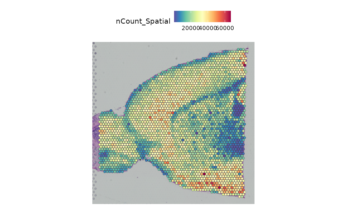

We normalize the data we use log normalization.

anterior1 <- NormalizeData(anterior1)

Running haystack on the spatial coordinates

The two inputs to singleCellHaystack are 1) the gene expression data and 2) the spatial coordinates of the Visium spots. Please note that we are not using an embedding as input space here, but the actual 2D coordinates of spots inside the tissue. Since this Visium dataset only contains about 2.7k spots and 12k genes, running singleCellHaystack should only take about a minute.

dat.expression <- GetAssayData(anterior1, slot = "data")
dat.coord <- GetTissueCoordinates(anterior1, "anterior1")

set.seed(123)
res <- haystack(dat.coord, dat.expression)
#> ### calling haystack_continuous_highD()...
#> ### Using package sparseMatrixStats to speed up statistics in sparse matrices.
#> ### Calculating row-wise mean and SD...
#> ### Filtered 0 genes with zero variance...
#> ### Using 100 randomizations...
#> ### Using 100 genes to randomize...
#> ### converting expression data from dgCMatrix to dgRMatrix
#> ### scaling input data...
#> ### deciding grid points...
#> ### calculating Kullback-Leibler divergences...
#> ### performing randomizations...
#> ### estimating p-values...
#> ### picking model for mean D_KL...
#> ### using natural splines
#> ### best RMSD  : 0.016
#> ### best df    : 5
#> ### picking model for stdev D_KL...
#> ### using natural splines
#> ### best RMSD  : 0.011
#> ### best df    : 9
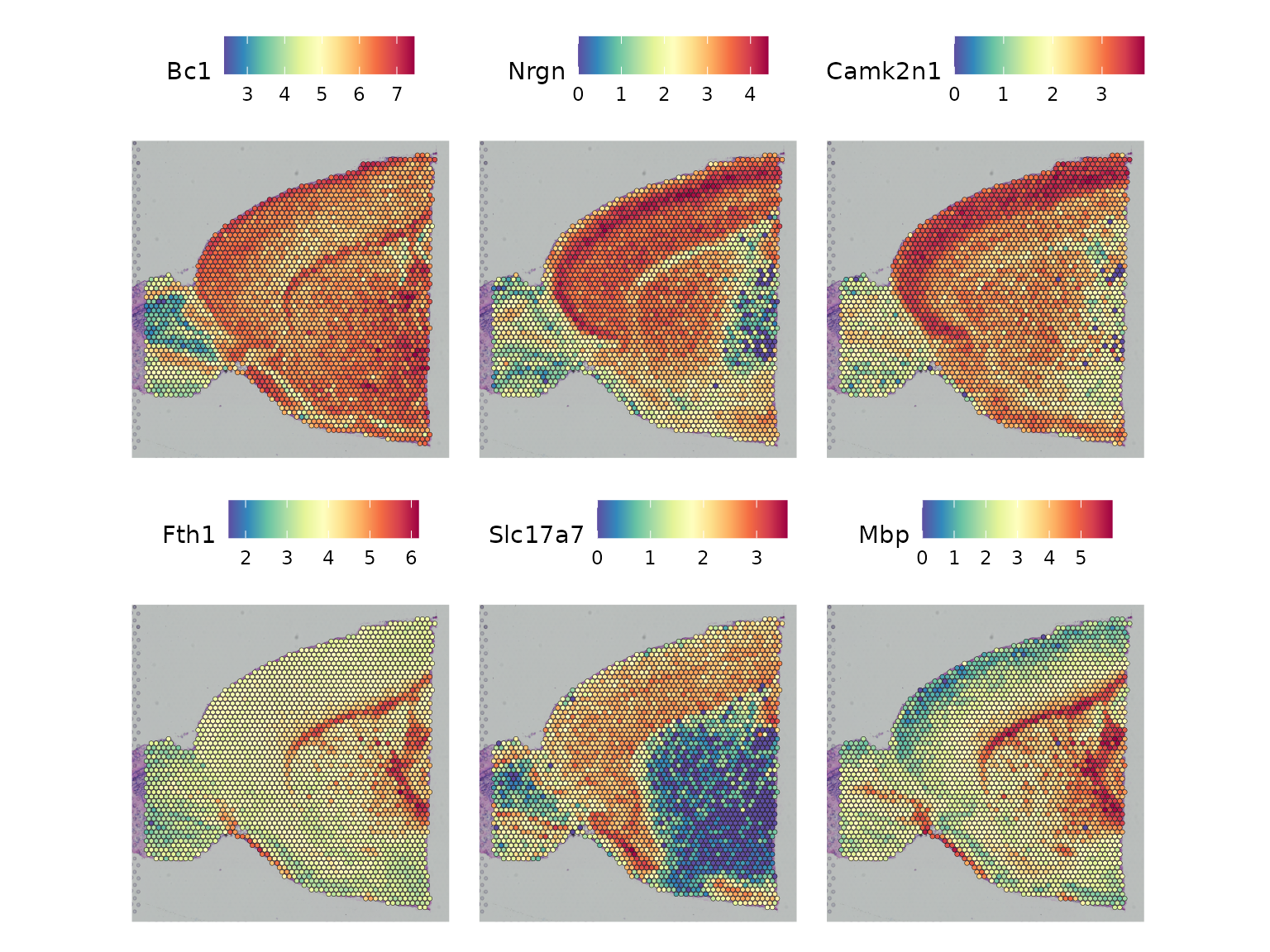
#> ### returning result...

We can check the top genes with spatial biased distribution.

show_result_haystack(res.haystack = res, n = 10)
#>                D_KL log.p.vals log.p.adj
#> Bc1     0.005965130  -137.7049 -133.6121
#> Nrgn    0.047198345  -137.0031 -132.9103
#> Camk2n1 0.021558345  -136.1950 -132.1022
#> Fth1    0.006648597  -132.1465 -128.0537
#> Slc17a7 0.175242409  -126.8016 -122.7088
#> Mbp     0.044803707  -125.1057 -121.0129
#> Penk    0.294461361  -124.8620 -120.7693
#> Nrn1    0.293755819  -122.9205 -118.8277
#> Cck     0.128716390  -122.8696 -118.7768
#> Pcp4    0.051290918  -121.5978 -117.5050

And we can visualize the expression of the 6 top-scoring genes in the spatial plot.

top6 <- show_result_haystack(res.haystack = res, n = 6)
SpatialFeaturePlot(anterior1, features = rownames(top6))